How to Create Sample Data Sets for Microsoft® Excel Spreadsheets

How to use Excel formulas, including the RANDBETWEEN, DATE and VLOOKUP functions, to quickly create meaningful sets of data for testing spreadsheets.

Last updated on 2024-04-29.

Preface

Your spreadsheets need thorough testing before they can be relied upon. Testing requires data. Those data need to be representative of the data that users will input when your spreadsheet goes live.

If your spreadsheet is to record sales of office stationery items, for example, then it's better if the data refer to “pencils”, “paper” and “erasers” than to generic lists like “Item 1”, “Item 2” and “Item 3”.

In this article are suggestions on how to produce data that your users will recognise, so that those users can be reliably engaged in testing.

This article introduces some functions to use in Excel formulas to create data values and provides some examples of how to create data sets; e.g. of dates, products, and people's names.

Excel's RANDBETWEEN Function

We'll use the RANDBETWEEN function extensively in creating data. RANDBETWEEN will return a whole number randomly drawn from between whatever lower and upper whole-number values you tell it:

RANDBETWEEN(lower_limit,upper_limit)

Note that in use RANDBETWEEN will change the value it produces each time you update your spreadsheet. So we'll need to suppress this action once our data set is complete.

Random Dates

Excel's built-in calendar treats dates as numbers. The number one stands for 1900-01-01; and the calendar increments by one for each day since then. So this formula would create a random number representing a date between 2019-01-01 and 2019-12-31:

=RANDBETWEEN(43466,43830)

To appreciate the numbers, put today's date in a cell (Ctrl + ;). Then apply the General number format to that cell.

Fiddling with actual numbers is a bit medieval. Using Excel's DATE function is much more now. DATE has this structure:

DATE(yyyy,mm,dd)

So, for a random date in 2019:

=RANDBETWEEN(DATE(2024,1,1),DATE(2019,12,31))

That's the formula you copy down the column in your data table headed “Invoice Date”, “Transaction Date”, “Date of Introduction” or whatever.

Item Data

Let's assume an Item could be a supplier, customer, product or service, and so on. Anything drawn from a list that you could input into Excel and use as the basis for a lookup table.

Here are the products from a company selling homes and wellbeing products for wild birds, input into Excel and provided with an ID number:

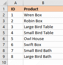
We give the cells A2 to B9 the range name nmProducts, which makes this formula easy to interpret:

=VLOOKUP(RANDBETWEEN(1,8),nmProducts,2)

How to Use the VLOOKUP Function in an Excel Formula explains the workings of VLOOKUP in detail.

The Data Set

Here's an Excel spreadsheet of data created using the formulas discussed above:

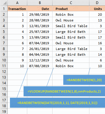
This data set is a small one. You can use the same approach to produce large sets — see People's Names below as an example.

Monetary Values

Costs are an example of values that you need to appear in your data to, say, two decimal places. Since RANDBETWEEN returns whole numbers only, you use this formula to achieve values to pounds and pence, or to dollars and cents:

=RANDBETWEEN(10000,1000000)/100

Perhaps, apply a currency format to the cells in your spreadsheets that use this formula.

Prices

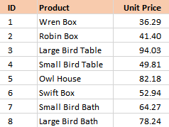
We usually tie prices to products and services. Our range name nmProducts now extends across three columns:

We're now challenged to have our product and its price for each transaction respond to the same random number.

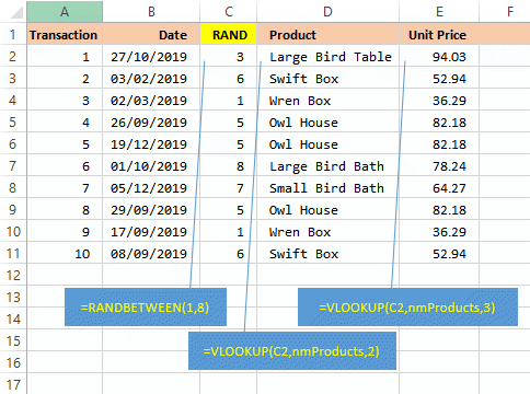
Here, both the Product and Unit Price column draw on the same random number generated in the RAND column.

Completing the Data Set

We now have techniques for producing random, yet meaningful, rows of data that could be adapted to generate data sets of any sort.

It just remains to freeze the data to remove the RANDBETWEEN functions that cause the data to change each time your spreadsheet recalculates.

But before doing that, I recommend you take a copy of the worksheet for future reference, so that you don't need to re-create the formulas each time you want a new data set.

To freeze the data, simply select it, Copy and Paste Values. Then you can delete the RAND column.

People's Names

One of the most common requests I receive is for sets of names for people. I've an instance of where 10,000 names were required for a data set.

Even if your requirement is for a few hundred only, even then you won't want to type them out. So, here is a suggestion for producing a data of almost any size set from scratch.

Start with a wordbook containing three worksheets as illustrated here:

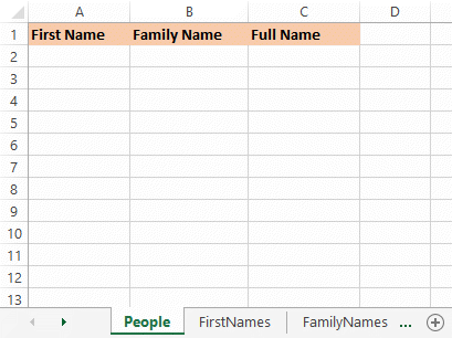
The People worksheet will contain the completed data set composed from entries in the other two sheets. Starting with the FirstNames sheet fill Column B with names. How?

Step One

Search the web for a free list of first name — e.g. https://github.com/smashew/NameDatabases/find/master.

Copy and paste the list into Column B —

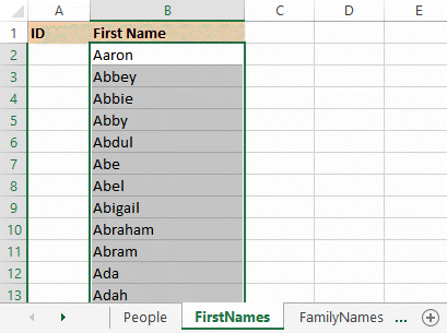
Step Two

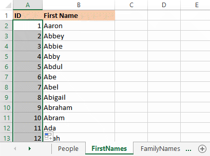
In Column A, number the names. This is one quick method:

1. Input the number one in Cell A2
2. Input the number two in A3
3. Select cells A2 and A3
4. Double-click the tiny handle at the bottom-right corner of your selection —

Step Three

Now apply a range name to your list. This name is to identify the cells starting at A2 and finishing at the bottom of the names in Column B. This is a method to achieve this:

1. Select Cell A2
2. Keyboard shortcut Shift+Ctrl+End
3. In the Name Box at the left-hand end of the Formula Bar, replace A2 with the input nmFirstNames. Press Enter to cement the range name in place —

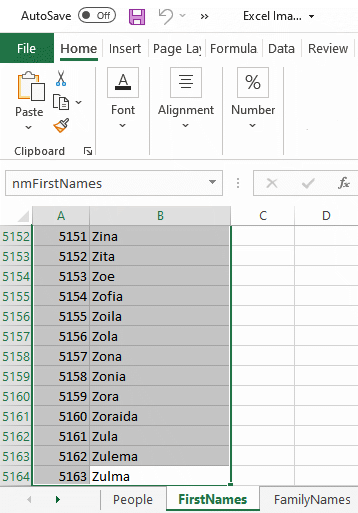
I always confirm my range naming has been successful:

1. Open the list of range names in the Name Box
2. Select from the list the name you want to check. Excel will select the block of cells it understands is spanned by that name
3. Repeat the keyboard shortcut Ctrl+. (that is, Ctrl + full stop) to move from corner to corner round the selection.

Now for the Family Names

Go to the FamilyNames worksheet and repeat the three steps, in Step Three applying the range name nmFamilyNames.

Completing the Names Data Set

These are the formulas in the People sheet that create your data set:

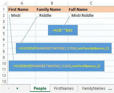
My download from the web of names yielded 5,163 first names and 3,706 family names. Hence the limits set in my RANDBETWEEN expressions.

Copy the formulas down as far as you need go to produce the number of names you want for your data set.

With my 5,163 by 3,706 lists, that's potential for 19,134,078 unique full names. Be that as it may, the formulas will not eliminate the possibility of duplicate full names.

If you don't want duplicates, copy Columns A, B and C and paste them as values into a new worksheet. Then you can use Excel's Remove Duplicates feature.

Your Support for DMW TIPS

Please support this website by making a donation to help keep it free of advertising and to help towards cost of time spent adding new content.

To make a contribution by PayPal in GBP (£ sterling) —

To make a contribution by PayPal in USD ($ US) —