Dropdown Lists in Microsoft® Excel Cells
On this page:
Last updated on 2024-05-02.
Purpose of Dropdown Lists
A dropdown list applied to a cell or group of cells on an Excel spreadsheet serves purposes including:
- Provision to users of an efficient method of inputting information
- Limitation of a user's choice of input to a proscribed list of values
- Removal of the risk of typos introducing mistakes into the spreadsheet during inputting.
Thoughtful deployment of drop-down lists contributes not only to spreadsheet accuracy but also to relief for users from possible anxiety over exactly what to input.
An Approach to Dropdown Lists
There's more than one method of creating a dropdown list in Excel. All of these are well covered on the web.
In this article I explain the method that I've found most useful for creating dropdown lists in the majority of my own spreadsheets and in spreadsheets I've created for clients.
The two-stage approach:
- Establish the list
- Create the dropdown, referencing that list.
With this approach, as I'll explain below, the list items are readily accessible: they are not buried in the construction of the dropdown.
List Preparation
I recommend this way to prepare your list:
- Create a worksheet in your workbook for the purpose of storing lists. (I name this worksheet “Lists”)
- In this worksheet create the list as you want it to appear in your dropdown, inputting items in cells down the same column. No empty cells
- Select the cells of the completed list. Then in Excel's Name Box type a name for that list. Be certain to complete your typing by pressing Enter
- Test that your range name is properly set by selecting it from the list of names appearing in the dropdown list of Excel's Name Box.
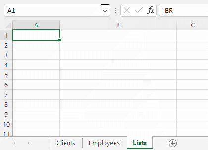
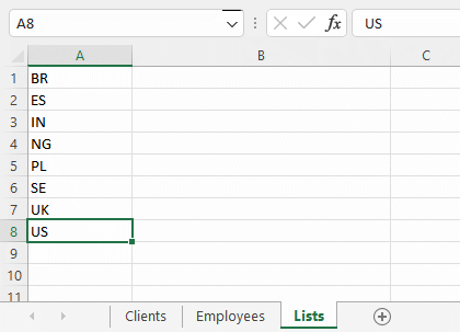
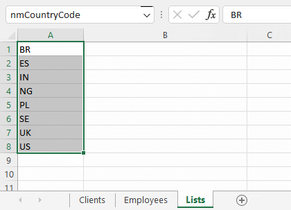
Such a name is what many Excel devotees refer to as a “range name”
In the screen clip above I've given the list of country codes the range name “nmCountryCode”
Now your list is ready for the dropdown to use. Remember its name for the next stage.
Creating the Dropdown
This is the way to create the dropdown:
- Select a cell to which you want the dropdown list to apply
- From Excel's ribbon choose the Data tab
- From the Data Tools section on that tab, choose Data Validation
- Under Settings in the Data Validation dialog box, select “List” from the Allow dropdown list
- In the Source box, type an equals sign followed by the range name you've given to your list. (Take care not to omit the equals sign)
- Click OK to close the dialog box.

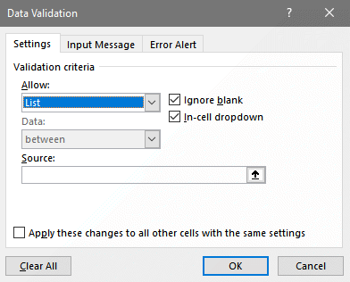
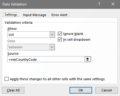
Your dropdown list should now be in place.
Applying the Dropdown List to Other Cells
Once you have your dropdown list applied to a cell, this is how to apply it to other cells:
- Select the cell containing the dropdown
- Issue the Copy command
- Select the cells to which you want to assign the dropdown list
- Issue the Paste Special command
- From the Paste Special dialog box, select the “Validation” option
- Click OK.
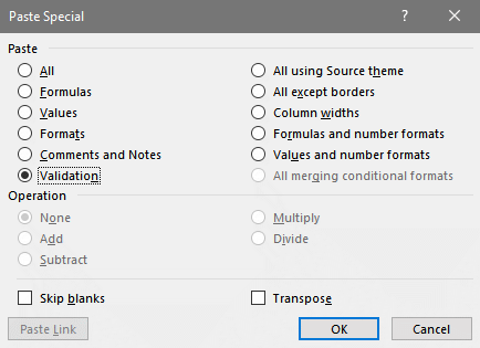
Your chosen cells should now be afforded the dropdown list.
Names for Dropdown Lists
I recommend avoiding using a range name for your list that Excel uses in its own workings. This will spare any confusion for users between, say, your choice of “Date” as a range name and Excel's “DATE” function.
In naming a list I always include a prefix of two or three lowercase letters in the name, e.g. “nm” as in “nmCountryCode”
This naming convention has the advantage of distinguishing range names of mine from those, like “Print_Area”, that Excel may have applied for its own purposes.
For spreadsheets in which I'm not the only person applying names to ranges of cells, I use my initials, “dmw”, as the prefix to distinguish my efforts.
Adding to a List
There are two circumstances to take into account when adding an item to a dropdown list:
1 – Item to be inserted into the list
Simply insert a new cell at the point in which you want the new item to appear, and input the item.
Nothing further needs doing: all the dropdowns in cells on your spreadsheet will now include this new item.
2 – Item to be added to the bottom of the list
When you've input a new item to the bottom of your list, you need to extend the range name to include it:
- Select the cell item in the list
- Choose the Formulas tab on Excel's ribbon and go to the Defined Names group
- Choose Name Manager to display the Name Manager dialog box
- In that dialog box, select the Name in question
- Click in the Refers to box at the bottom of the dialog box
- On the spreadsheet, select the list cells including the new one
- Click the ✔
- Click Close
- Test that your range name is properly set by selecting it from the list of names appearing in the dropdown list of Excel's Name Box.
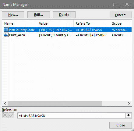
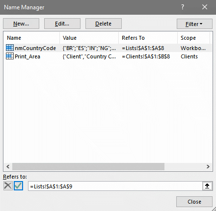
Excel will select the sells currently providing your list
Cautionary Note — Changing an Item in a List
If you change an item in your list — e.g. from “Streich-Waters” to “Streich-Waters LLP”— then that change will not update any of the cells in your spreadsheet containing the original list item.
This means that you'll need to adjust entries already recorded in your spreadsheet before anyone uses it with the revised dropdown list.
Cautionary Note — Deleting an Item from a List
If you delete an item from your list, then that item will not disappear from any of the cells in your spreadsheet to which originally you applied it using the dropdown.
This means that you'll need to adjust entries already recorded in your spreadsheet before anyone uses it with the revised dropdown list.
Your Support for DMW TIPS
Please support this website by making a donation to help keep it free of advertising and to help towards cost of time spent adding new content.
To make a contribution by PayPal in GBP (£ sterling) —
To make a contribution by PayPal in USD ($ US) —
