How to Use Microsoft® Excel's VLOOKUP Function

Last updated on 2024-05-15.

When to Use VLOOKUP

You have a list from which you need to pick information relating to a particular entry in that list. VOOKUP saves you the chore of manually copy and pasting from the list or of typing values afresh.

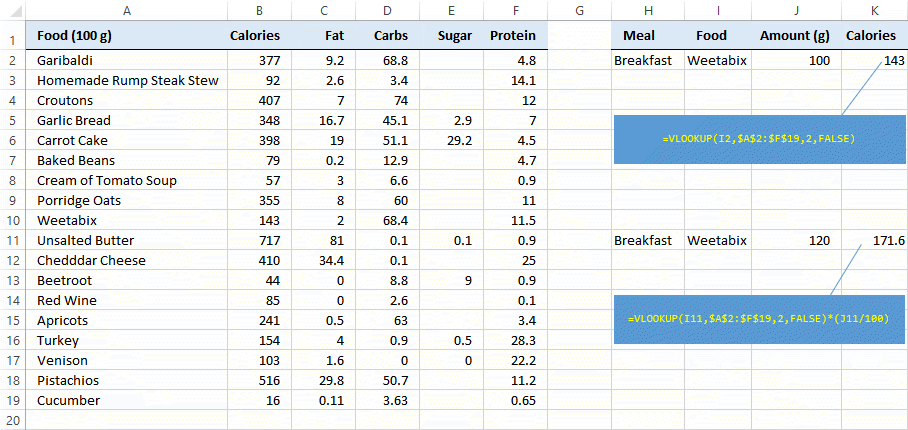
For example, you're maintaining a Daily Food Consumption spreadsheet. As you input Weetabix as part of a breakfast, you want the spreadsheet to look up automatically the calorific value of Weetabix in this, your reference list of nutritional values:

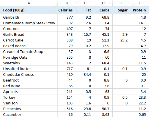
So, when you enter a breakfast including Weetabix into your spreadsheet you want it to pick up on the fact you've laid in 143 calories for each 100 g of breakfast cereal you've eaten.

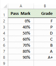
Another example: you are recording test scores and need each one represented as a grade.

So, if Poppi scores 67% in her science paper you want VLOOKUP to register that as a “C” grade.

In this example you want VLOOKUP to find a best-fit, rather than an exact match, between mark and grade.

One thing these two lists, and any other list you want to use, must have in common is that their left-most columns are the ones that contain the values amongst which VOOKUP is to seek a match.

A facet of VLOOKUP itself is that it can look for exact matches — e.g. “Weetabix” — or best-fits, as with Poppi's 67%.

How VLOOKUP Works

VOOKUP needs four pieces of information — referred to as its arguments — in order to do its business:

value to look up This is the value — text, number, date, etc — which you want VLOOKUP to locate in your list.

where to look up This is the range of cells constituting the list from which VLOOKUP is to return a result.

list's results column Within the list, this is the column — counting from the left — from which you want VOOKUP to pick out the value to return to your spreadsheet. The left-hand column counts as column one.

approximate or exact match This is the instruction to VLOOKUP to make either an exact match with items in the list or a best fit.

Note If you need an exact match, then the order of items in the left-most column of your list does not matter. If, on the other hand, you want a best fit, then the list items must be in ascending order.

Examples of VLOOKUP Formulas

Best-fit Matches

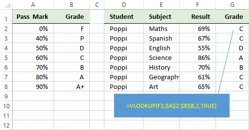
=VLOOKUP(F2,$A$2:$B$8,2,TRUE), the formula in Cell G2 in the spreadsheet above, takes Poppi's 69% result from Cell F2 and looks it up in left-hand column of the Grades list $A$2:$B$8.

2 tells VLOOKUP to return a value from the second column in the list.

TRUE tells VLOOKUP to find a best-fit for 69% in the left-hand column of the list. 69% falls within the 60% to 70% Grace C band. Had Poppi achieved 70%, then that would have fallen within the Grade B band.

Exact Matches

In both the formulas for breakfast, VLOOKUP has FALSE as its fourth argument, driving it to make an exact match.

For the 120 g breakfast, the complete VLOOKUP is multiplied by the fraction that makes the result of the formula as a whole fit a breakfast of that weight.

Use of Named Ranges

In many many instances the application of names to ranges of cells makes formulas easier to compose, understand and maintain. I recommend the use of range names in all VLOOKUP formulas.

Taking this spreadsheet as an example, it uses the fixed reference $A$2:$B$8 as the second argument of its VLOOKUP formula:

To replace that reference with a range name, we first of all have to create the name, say nmGrades. We select the list of Pass Marks and Grades, type the name into Excel's Name Box and press Enter:

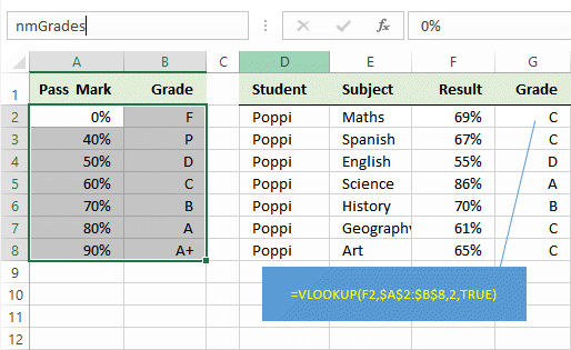
Note that our range spans the marks and grades only, not the column headings.

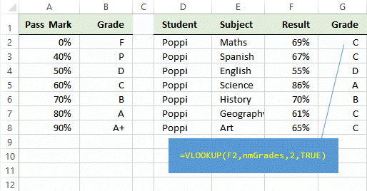
Now we can edit the formula to replace $A$2:$B$8 by nmGrades:

VLOOKUPs Across Two Spreadsheets

Worksheets in Same Workbook

If you range name your list before you compose your formulas, then creating a VLOOKUP formula is the same as usual:

1. In the cell in which you want the result, commence you formula with =VLOOKUP(B2) (replacing B2 with what's appropriate for your formula)
2. To extend your formula to, for example, =VLOOKUP(B2,nmGrades), type the name you've given to the range of cells comprising your list

OR

From Excel's ribbon choose the Formulas tab, then from the Define Names group drop-down the Use in Formula list and select the range name

3. Complete the formula and then press Enter.

Worksheets in Different Workbooks

Have both workbooks open. It helps of you have already saved them so that you have meaningful names by which to identify them.

1. In the cell in which you want the result, commence your formula with =VLOOKUP(B2), (replacing B2 with what's appropriate for your formula)
2. To extend your formula to, for example, =VLOOKUP(B2,nmGrades), move the focus to the workbook that contains your list
3. =VLOOKUP(O4,Database.xlsm!nmGrades)
4. Complete your formula, =VLOOKUP(O4,Database.xlsm!nmGrades,2,FALSE) and press Enter.

Like mine, your formula will include your equivalent of Database.xlsm!nmGrades. The stuff to the left of the ! — Database.xlsm — is the pointer to the supporting workbook.

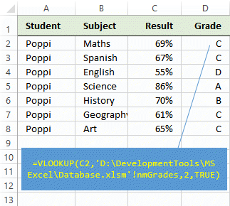If you close both workbooks, saving them as you do so, and then open only the one with the VLOOKUP formula in it, you'll note that the formula points to the whereabouts of the supporting workbook.

Take care not to move the supporting workbook from where your formula expects it to reside.

Your Support for DMW TIPS

Please support this website by making a donation to help keep it free of advertising and to help towards cost of time spent adding new content.

To make a contribution by PayPal in GBP (£ sterling) —

To make a contribution by PayPal in USD ($ US) —