How to Total Percentages in Microsoft® Excel

“I have a column of figures, each of which I want to display as the percentage of the total. Sometimes the total of the percentages does not come to 100% depending on the figures. Is there a way round this?”

Last updated on 2024-05-03.

Illustrating the Problem

This is a challenging problem that I meet in various guises. I keep trying to find the ideal way of tackling it; but, even with the method I describe here, I don't consider I have fully achieved that aim yet.

This spreadsheet illustrates your question:

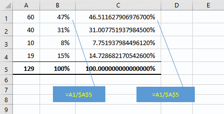
The formulas in Cells B1 and C1 (copied to rows two to four) is this:

=A1/$A$5

Percentage formatting is applied to Columns B and C. Formatting applied to Column B restricts the display of percentages to whole numbers; to Column C, to 15 decimal places.

Created with AutoSum, the total neither in Cell B5, nor in Cell C5, is correct. The rounding effects of formatting on Column B, introduce significant errors in presentation such as that in Column B.

In Column C we come up against the amount of precision with which Excel can store numbers: 15 digits.

A Possible Solution

In my solution, we need two columns, B and C here (usually Column C would be hidden):

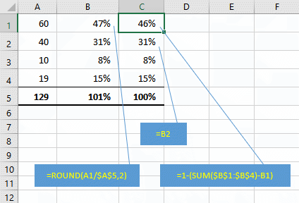
The formula in cell B1 (copied to the other cells as far as row 4) is this:

=ROUND(A1/$A$5,2).

Note that you round to two decimal places when you want to display resultant percentages with no decimal places. If you want to display to one decimal place, use this formula:

=ROUND(A1/$A$5,3).

The formula in cell C1 is this:

=1-(SUM($B$1:$B$4)-C1)

Formulae in rows two to four in this column are all the same:

=B2

What all this achieves is to apply a fudge factor to the result in cell C1.

A down side of this technique is that anyone reading your spreadsheet and checking your figures with a calculator will not be able to duplicate your results.

Furthermore, if the value in cell A1 is relatively small, the fudge factor will introduce a substantial percentage error in the value in cell C1. I've not found a formula that automatically will apply the fudge factor to the largest value in column A.

Applying a fudge factor is the only way I can find to make your percentages total 100%. I've left the challenge of finding a superior solution to my subconscious.

Targeting the Fudge

The closing two paragraphs of the section above express my concern over the technique described — the strong possibility of substantial errors when the fudge factor is applied to a value that low in comparison to others:

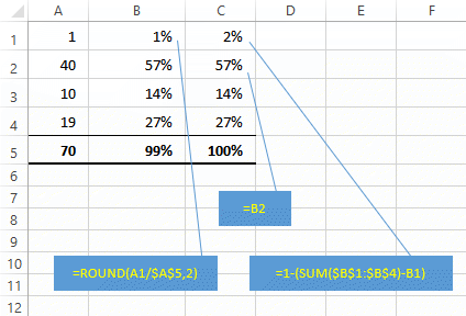
In the above the error is an extreme 50% accruing in Row 1.

Well, taking my own advice, I left the conundrum to my subconscious, which dutifully brought the following suggestion to my attention:

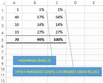
Examining the formula in Cell C1, which is copied down Column C:

=IF(A1=MAX($A$1:$A$4),1-(SUM($B$1:$B$4)-B1),B1)

The IF uses A1=MAX($A$1:$A$4) to examine the value in Cell A1 to determine whether or not that value is the greatest in the range of Cells A1 to A4. If it's the greatest, then the 1-(SUM($B$1:$B$4)-B1) fudge factor is the result of the formula; if it's not, then the value in Cell B1 is the result.

Things looked promising until testing with the same value accorded to two cells in Column A:

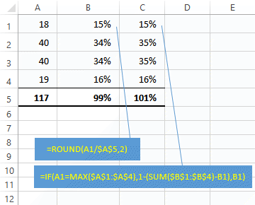
Returning this new challenge to my subconscious, I'm half anticipating it's going to point me towards using VBA.

Your Support for DMW TIPS

Please support this website by making a donation to help keep it free of advertising and to help towards cost of time spent adding new content.

To make a contribution by PayPal in GBP (£ sterling) —

To make a contribution by PayPal in USD ($ US) —

Thanks, in anticipation.