How to Create Criteria for Microsoft® Excel DSUM Formulae

Last updated on 2024-05-02.

Question

“We are running a database in Excel and want to use the DSUM function to calculate totals over ranges of dates on a month-by-month basis. This means we have to set up a DSUM formula for each month and this we are doing longhand at the moment. Is there a way we can set up a formula that we can copy to save us all the longhand work?”

When you have a database in an Excel spreadsheet, the DSUM function can calculate totals from the data according to the criteria with which you supply it.

Application of DSUM

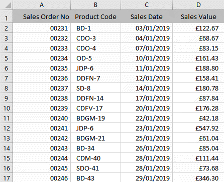
This screen dump illustrates the data in the table (much simplified!) upon which you want your DSUM formula to work:

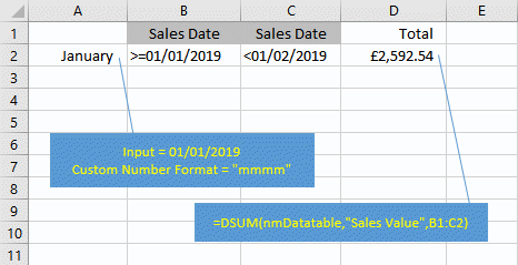
And this one shows how you have set up the criteria in columns B and C, used by the DSUM formulae in column D:

The formula in cell D2 is assumes that you use the range name nmDatatable applied to all the data in your main table:

=DSUM(nmDatatable,"Sales Value",B1:C2)

It's imperative that in the construction of your DSUM formula you use exactly the names appearing as column headings in your data table.

Preparing for Future Months and Years

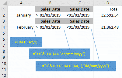
You now prepare February's criteria so that you can copy it down your spreadsheets to produce criteria for March onwards.

What you want to be able to do is copy the last month's block of cells to create a new month (that is, copy the A5:D6 block to cell A7 to create a block for April).

Cell A4's formula uses the EDATE function which advances by one month any date you give it. Here, EDATE advances the date in Cell A2 to 01/02/2019.

The TEXT function in Cell B4 examines the content of Cell A4 and renders it as a string of text in the dd/mm/yyyy format. Concatenate that string with >= to produce the criterion.

In Cell C4, your formula combines TEXT and EDATE functions to produce February's second Sales Date crierion.

Complete February's calculations by copying Cell D2's formula to Cell C4 to provide a Total.

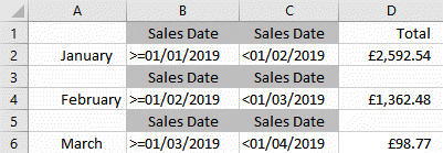
The range of cells A3:D4 is the template each month from March onwards. Simply copy that range, and paste it down the worksheet:

Hiding columns B and C, and all the odd-numbered rows, results in a neat summary:

For other years, simply input 01/01/2020, or 01/01/2018, as appropriate in Cell A2.

Your Support for DMW TIPS

Please support this website by making a donation to help keep it free of advertising and to help towards cost of time spent adding new content.

To make a contribution by PayPal in GBP (£ sterling) —

To make a contribution by PayPal in USD ($ US) —

Thanks, in anticipation.

Disclaimer

David Wallis does not accept any liability for loss or damage to data to which any techniques, methods or code included in this website are applied. Back up your data; test thoroughly before using on live data.