How to Create an Adaptable Conditional Format in Excel
Last updated on 2024-05-02.
Introduction
Consider that you need a conditional format to highlight cells that contain numeric values higher and lower than certain values, as in this spreadsheet:
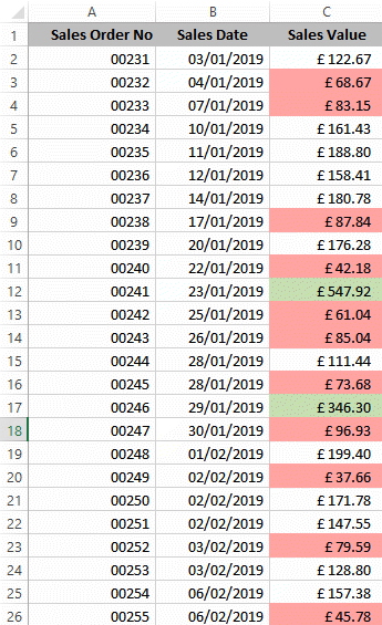
The background colours are used to distinguish values that are higher than £300.00 and lower than £100.00 limits.
Sometimes, in a spreadsheet like this one, you need to change these limits. If you've embedded these limits in your definitions of the formats, then you have to edit those formats each time you want to apply new limits. This can be a chore and time consuming.
Furthermore, you may want to let users of the spreadsheet set the limits, but you know they wouldn't be comfortable editing conditional formats for themselves.
This article describes one way of addressing these issues.
Setting Up
Before composing the conditional formats, we need two cells that are to contain the limits. Like this:
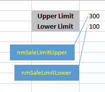 These cells can be anywhere in the workbook that suits you — see Where to Set the Limits.
The cells that contain the limits have been given the range names nmSalesLimitUpper and nmSalesLimitLower.
If you or any user moves these cells, then these names will follow the move.
The conditional formats reference these cells by name. So, when the limits need to change, the new values are input into these cells. The formats will adjust to them automatically.
Composing the Conditional Formats
We need two conditional formats, one to manage the upper limit, the other the lower. Starting with the format for the upper limit:
1. Select the cells to which you want your format to apply. (In the spreadsheet illustrated in the Introduction, these are the cells in the range C2:C26)
2. From the Home tab on Excel's ribbon, click on Conditional Formatting to display this pane:
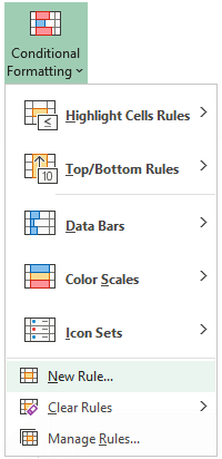
3. Choose New Rule to display the New Formatting Rule dialog box:
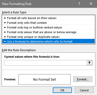
4. Choose Use a formula to determine which cell to format from the list of Rule Types.
5. In the Format values where this formula is true box, input =C2>=nmSaleLimitUpper, where C2 is the address of the cell that starts the block of cells to which the formatting is to apply.
6 Click Format and set the formatting for cells containing values in the upper band. (I've done no more than prescribe a green background fill):
7. Click OK.
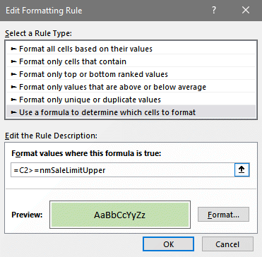
8. Keep selected the cells to be formatted and repeat steps #2 to #7, but at step #5, input =C2<nmSaleLimitLower.
Modifying a Conditional Format
If you need to alter the formats you've created, then from the Home tab on Excel’s ribbon, click on Conditional Formatting and click Manage Rules at the bottom of the list to display the Conditional Formatting Rules Manager dialog box:
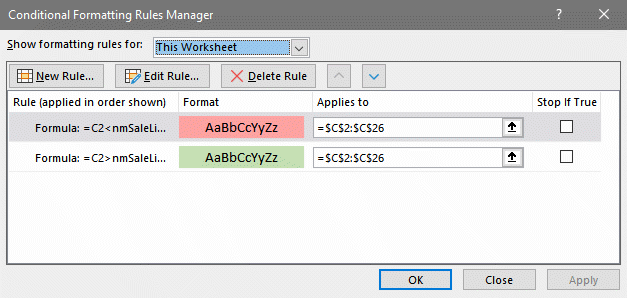
Select the rule you want to change, and click Edit Rule.
Where to Set the Limits
You may place the cells that contain the limits anywhere in your workbook.
I've settled on placing these in a worksheet dedicated to values used in formulas in the workbook. This approach makes it easy for me to locate any value in use; I don't waste time hunting them down, as used to happen when I scattered them throughout workbooks.
Giving this worksheet a name such as References identifies its purpose. I always know where to tell users to go to change values.
Your Support for DMW TIPS
Please support this website by making a donation to help keep it free of advertising and to help towards cost of time spent adding new content.
To make a contribution by PayPal in GBP (£ sterling) —
To make a contribution by PayPal in USD ($ US) —
